| Oracle® OLAP Application Developer's Guide, 10g Release 2 (10.2) Part Number B14349-05 |
|
|
PDF · Mobi · ePub |
| Oracle® OLAP Application Developer's Guide, 10g Release 2 (10.2) Part Number B14349-05 |
|
|
PDF · Mobi · ePub |
A cube always returns summary data to a query as needed. While the cube may store data at the day level, for example, it returns a result at the quarter or year level without requiring a calculation in the query. This chapter explains how to optimize the unique aggregation subsystem of Oracle OLAP to provide the best performance for both data maintenance and querying.
This chapter contains the following topics:
Aggregation is the process of consolidating multiple values into a single value. For example, data can be collected on a daily basis and aggregated into a value for the week, the weekly data can be aggregated into a value for the month, and so on. Aggregation allows patterns in the data to emerge, and these patterns are the basis for analysis and decision making. When you define a data model with hierarchical dimensions, you are providing the framework in which aggregate data can be calculated.
Aggregation is frequently called summarization, and aggregate data is called summary data. While the most frequently used aggregation operator is Sum, there are many other operators, such as Average, First, Last, Minimum, and Maximum. Oracle OLAP also supports weighted and hierarchical methods. Following are some simple diagrams showing how the basic types of operators work. For descriptions of all the operators, refer to "Aggregation Operators" .
Figure 8-1 shows a simple hierarchy with four children and one parent value. Three of the children have values, while the fourth is empty. This empty cell has a null or NA value. The Sum operator calculates a value of (2 + 4 + 6)=12 for the parent value.
Figure 8-1 Summary Aggregation in a Simple Hierarchy

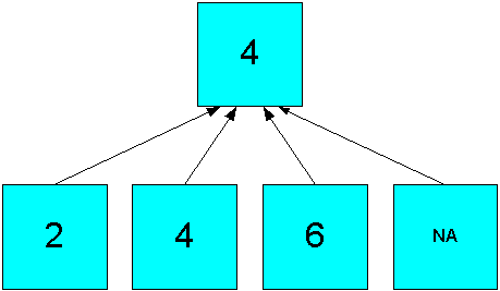
The Average operator calculates the average of all real data, producing an aggregate value of ((2 + 4 + 6)/3)=4, as shown in Figure 8-2.
Figure 8-2 Average Aggregation in a Simple Hierarchy
The hierarchical operators include null values in the count of cells. In Figure 8-3, the Hierarchical Average operator produces an aggregate value of ((2 + 4 + 6 +NA)/4)=3.
Figure 8-3 Hierarchical Average Aggregation in a Simple Hierarchy

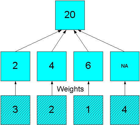
The weighted operators use the values in another measure to generate weighted values before performing the aggregation.Figure 8-4 shows how the simple sum of 12 in Figure 8-1 changes to 20 by using weights ((3*2) + (2*4) + (NA*6) +(4*NA)).
Figure 8-4 Weighted Sum Aggregation in a Simple Hierarchy
Analytic workspaces provide an extensive list of aggregation methods, including weighted, hierarchical, and weighted hierarchical methods.
The following are descriptions of the basic aggregation operators:
Average: Adds non-null data values, then divides the sum by the number of data values that were added together.
First Non-NA Data Value: Returns the first real data value.
Last Non-NA Data Value: Returns the last real data value.
Maximum: Returns the largest data value among the children of each parent.
Minimum: Returns the smallest non-null data value among the children of each parent.
Nonadditive: Does not aggregate the data.
Sum: Adds data values.
These are the scaled and weighted aggregation operators.
These operators require a measure providing the weight or scale values in the same cube. In a weight measure, an NA (null) is calculated like a 1. In a scale measure, an NA is calculated like a 0.
The weighted operators use outer joins, as described in "When Does Aggregation Order Matter?".
Scaled Sum: Adds the value of a weight object to each data value, then adds the data values.
Weighted Average: Multiplies each data value by a weight factor, adds the data values, and then divides that result by the sum of the weight factors.
Weighted First: Multiplies the first non-null data value by its corresponding weight value.
Weighted Last: Multiplies the last non-null data value by its corresponding weight value.
Weighted Sum: Multiplies each data value by a weight factor, then adds the data values.
The following are descriptions of the hierarchical operators. They include all cells identified by the hierarchy in the calculations, whether the cells contain data or not .
Hierarchical Average and the Hierarchical Weighted operators use outer joins.
Hierarchical Average: Adds data values, then divides the sum by the number of the children in the dimension hierarchy. Unlike Average, which counts only non-null children, hierarchical average counts all of the logical children of a parent, regardless of whether each child does or does not have a value.
Hierarchical First Member: Returns the first data value in the hierarchy, even when that value is null.
Hierarchical Last Member: Returns the last data value in the hierarchy, even when that value is null.
Hierarchical Weighted Average: Multiplies non-null child data values by their corresponding weight values, then divides the result by the sum of the weight values. Unlike Weighted Average, Hierarchical Weighted Average includes weight values in the denominator sum even when the corresponding child values are null.
Hierarchical Weighted First: Multiplies the first data value in the hierarchy by its corresponding weight value, even when that value is null.
Hierarchical Weighted Last: Multiplies the last data value in the hierarchy by its corresponding weight value, even when that value is null.
The OLAP engine aggregates a cube across one dimension at a time. When the aggregation operators are the same for all dimensions, the order in which they are aggregated may or may not make a difference in the calculated aggregate values, depending on the operator.
You should specify the order of aggregation when a cube uses multiple aggregation methods. The only exceptions are that you can combine Sum and Weighted Sum, or Average and Weighted Average, when the weight measure is only aggregated over the same dimension. For example, a weight measure used to calculate weighted averages across Customer is itself only aggregated across Customer.
The weight operators are uncompressible for the specified dimension and all preceding dimensions. For a compressed cube, you should list the weighted operators as early as possible to minimize the number of outer joins. For example, suppose that a cube uses Weighted Sum across Customer, and Sum across all other dimensions. Performance is best if Customer is aggregated first.
The following information provides guidelines for when you must specify the order of the dimensions as part of defining the aggregation rules for a cube.
When these operators are used for all dimension of a cube, the order does not affect the results:
Maximum
Minimum
Sum
Hierarchical First Member
Hierarchical Last Member
Hierarchical Average
Even though you can use the Sum and Maximum operators alone without ordering the dimensions, you cannot use them together without specifying the order. The following figures show how they calculate different results depending on the order of aggregation. Figure 8-5 shows a cube with two dimensions. Sum is calculated first across one dimension of the cube, then Maximum is calculated down the other dimension.
Figure 8-5 Sum Method Followed by Maximum Method
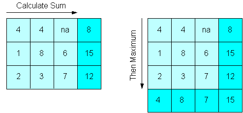
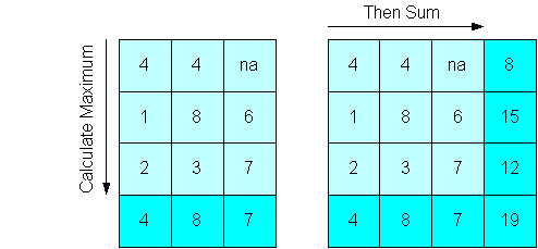
Figure 8-6 shows the same cube, except Maximum is calculated first down one dimension of the cube, then Sum is calculated across the other dimension. The maximum value of the sums in Figure 8-5 is 15, while the sum of the maximum values in Figure 8-6 is 19.
Figure 8-6 Max Method Followed by Sum Method
Compressed composites are used to store extremely sparse data. Use this aggregation strategy for compressed cubes:
Identify the dimension with the most members. If several dimensions have about the same number, then choose the dimension with the most levels. Do not pre-aggregate this dimension.
Pre-aggregate all other dimensions up to, but not including, the top level, unless the next level down has a large number of members.
You can adjust these basic guidelines to the particular characteristics of your data. For example, you may skip levels that are seldom queried from pre-aggregation. Or you may need to pre-aggregate a level with a large number of child values, to provide acceptable run-time performance.
Uncompressed cubes are used to store data that is either moderately sparse or dense. The strategy for aggregating noncompressed cubes is called skip-level aggregation, because some levels are stored and others are skipped until runtime. The success of this strategy depends on choosing the right levels to skip, which are those that can be calculated quickly in response to a query.
As a general rule, you should skip levels for only one or two dimensions and for no more than half of the dimensions of the cube. Choose the dimensions with the most levels in their hierarchies for skip-level aggregation.
Slower varying dimensions take longer to aggregate because the data is scattered throughout its storage space. If you are optimizing for data maintenance, then fully aggregate the faster varying dimensions and use skip-level aggregation on the slower varying dimensions.
You can identify the best levels to skip by determining the ratio of dimension members at each level, and keeping the ratio of members to be rolled up on the fly at approximately 10:1 or less. This ratio assures that all answer sets can be returned quickly. Either a data value is stored in the analytic workspace so it can simply be retrieved, or it can be calculated quickly from 10 stored values.
This 10:1 rule is best applied with some judgment. You might want to permit a higher ratio for levels that you know are seldom accessed. Or you might want to store levels at a lower ratio if you know they have heavy use. Generally, you should strive for a lower ratio instead of a higher one to maintain the best performance.
Aggregation rules identify how and when the aggregate values are calculated. You define the aggregation rules for each cube, and you can override these rules by defining new ones for a particular measure.
The aggregation rules defined for a cube or a measure are always performed over all dimension members. You can perform a partial aggregation only in a calculation plan and only for regular composites.
Note:
Do not set status for a compressed cube. All members must be in status.To aggregate over a portion of a measure, you select the dimension members that identify the cells containing the source data, using the Status page of the Aggregation property sheet. You do not need to select the target cells. All of the cells identified by the ancestors of the selected dimension members are aggregated, either when you execute the cube script or when a user queries the measure.
When you select the dimension members, they are in status. This means that the dimension members have been selected for use in a calculation, a query, or other data manipulation. Likewise, out of status means that the dimension members have been excluded from use.
Figure 8-7 shows an aggregation in which the 12 months of 2006 are in status. Neither the quarters nor the year are in status, but aggregates are generated for all levels.
Figure 8-7 Sum Aggregation With All Source Values in Status
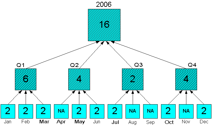
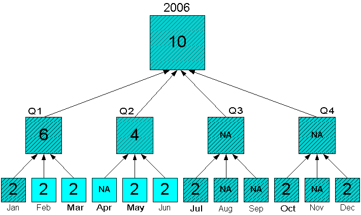
Figure 8-8 shows the same portion of data, but with only Feb to Jun in status. Aggregates are calculated only for Q1, Q2, and 2006. Note that Jan is included in the aggregation, even though it is out of status. The aggregation engine adds the ancestors, then the children to status before aggregating the data, as a means of maintaining the integrity of the data. The values for Q3 and Q4 are not included in the aggregation.
Figure 8-8 Sum Aggregation With Some Source Values Out of Status
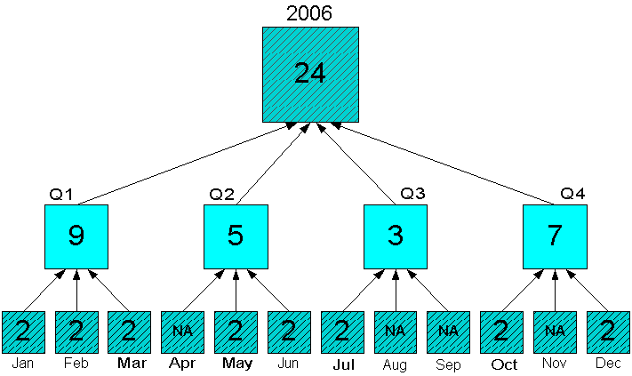
You may need to aggregate data that is stored in the middle of a hierarchy, perhaps if the data for a particular measure is not available or needed at the base level. You must be sure that the cells with the data are the lowest levels in the hierarchy in status. Figure 8-9 shows quarterly forecast data in status and aggregated to the year. The monthly values are not in status, and thus are excluded from the aggregation.
Figure 8-9 Sum Aggregation From the Quarterly Level
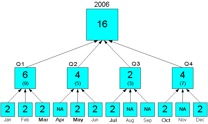
Aggregation begins at the lowest level in status and rolls up the hierarchy. The aggregate values overwrite any pre-existing values higher in the hierarchy. Figure 8-10 shows that when the Month level is in status, those values overwrite the forecast values at the Quarter level. The status of Quarter and Year has no effect on the aggregation.
Figure 8-10 Sum Aggregation From the Month Level Overwrites Quarters
The previous guidelines provide an approach to aggregation that should help you meet these basic goals:
If you anticipate problems with one or more of these goals, then you should keep them in mind while devising your aggregation rules. Otherwise, you may need to make adjustments after the initial build, if you experience problems meeting all of these goals.
Often the problem can be solved by changing factors other than the aggregation rules, as described in the following topics.
Note:
Be sure to run the Sparsity Advisor so that the data is structured in the most efficient way. Refer to "Choosing a Data Storage Strategy".Most organizations allocate a batch window in which all data maintenance must be complete. If you are unable to finish refreshing the data in the allotted time, then you can make the following adjustments.
Be sure that you have set the database initialization parameters correctly for data maintenance, as described in "Setting Database Initialization Parameters". You can make significant improvements in build performance by setting SGA_TARGET, PGA_AGGREGATE_TARGET, and JOB_QUEUE_PROCESSES.
After the initial build, you can save time by aggregating only newly loaded values, instead of aggregating all of them again. Partial aggregation is a choice you can make in the Maintenance Wizard.
Analytic workspaces are stored in partitioned tables, and you can create partitioned cubes. You can use these partitions to distribute the data across several disks, thus avoiding bottlenecks in I/O operations.
See Also:
Chapter 12, "Administering Oracle OLAP"Your analytic workspace must fit within the allocated resources. The more levels of aggregate data that you store, the larger the tablespaces must be to store the analytic workspace.
The data type is an important consideration when estimating the size of an analytic workspace. The most commonly used data types for measures are NUMBER and DECIMAL. The difference in size is significant: an unscaled NUMBER value is 22 bytes and a DECIMAL value is 8 bytes.
An analytic workspace must provide good performance for end users. When pre-aggregation is done correctly, the response time for queries does not noticeably slow down. Analytic workspaces are optimized for multidimensional calculations, so that run-time summarizations should be extremely fast. However, runtime performance suffers if the wrong choices are made.
If response time is poor, then review the decisions you made in skipping levels and find those that should be pre-aggregated. Try to identify and pre-aggregate those areas of the data that are queried heavily. Check the level on which you partitioned the cube. Remember that all levels above the partition are calculated on the fly. When partitioning over Time, the Month level is a much better choice than Day.
Read the recommendations given in the previous topics. The savings in maintenance time and disk storage may be used to pre-aggregate more of the data.