| Oracle® OLAP Application Developer's Guide, 10g Release 2 (10.2) Part Number B14349-05 |
|
|
PDF · Mobi · ePub |
| Oracle® OLAP Application Developer's Guide, 10g Release 2 (10.2) Part Number B14349-05 |
|
|
PDF · Mobi · ePub |
This chapter explains how to design a dimensional data model and create dimensions and cubes using Analytic Workspace Manager.
This chapter contains the following topics:
Chapter 1 introduced the dimensional objects: Cubes, measures, dimensions, levels, hierarchies, and attributes. In this chapter, you learn how to define them in Oracle Database, but first you must decide upon the dimensional model you want to create. What are your measures? What are your dimensions? How can you distinguish between a dimension and an attribute in your data? You can design a dimensional model using pencil and paper, a database design software package, or any other method that suits you.
If your source data is already in a star or snowflake schema, then you already have the elements of a dimensional model:
Fact tables correspond to cubes.
Data columns in the fact tables correspond to measures.
Foreign key constraints in the fact tables identify the dimension tables.
Dimension tables identify the dimensions.
Primary keys in the dimension tables identify the base-level dimension members.
Parent columns in the dimension tables identify the higher level dimension members.
Columns in the dimension tables containing descriptions and characteristics of the dimension members identify the attributes.
You can also get insights into the dimensional model by looking at the reports currently being generated from the source data. The reports identify the levels of aggregation that interest the report consumers and the attributes used to qualify the data.
While investigating your source data, you may decide to create relational views that more closely match the dimensional model that you plan to create.
See Also:
"Overview of the Dimensional Data Model" for an introduction to dimensional objects
Appendix A, "Designing a Dimensional Model," for a case study of developing a dimensional model for the Global analytic workspace
Your goal in using Analytic Workspace Manager is to create a multidimensional data store that supports business analysis. Analytic Workspace Manager is the primary tool for creating, developing, and managing analytic workspaces. The main window provides two views: the Model View and the Object View. You can switch between views using the View menu. In addition, there are menus, a toolbar, a navigation tree, and property sheets. When you select an object in the navigation tree, the property sheet to the right provides detailed information about that object. When you right-click an object, you get a choice of menu items with appropriate actions for that object.
Analytic Workspace Manager has a full online Help system, which includes context-sensitive Help.
The Model View enables you to define a multidimensional model composed of dimensions, levels, hierarchies, attributes, measures, calculated measures, and measure folders. The model is stored in the analytic workspace as database standard form metadata.
A drag-and-drop user interface facilitates mapping of the objects to columns in relational tables, views, and synonyms in Oracle Database. The source columns can be star, snowflake, or any other schema design that supports the multidimensional model.
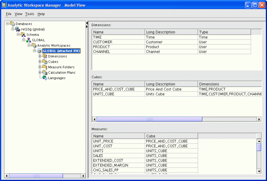
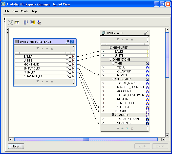
Figure 3-1 shows the dimensions, cubes, and measures created in the GLOBAL analytic workspace.
Figure 3-1 Model View in Analytic Workspace Manager
The Object View provides a graphical user interface to the OLAP DML. You can create, modify, and delete individual workspace objects. This view is provided for users who are familiar with the OLAP DML and want to upgrade from Express databases or modify custom applications. You should not use this view to manually change a standard form analytic workspace, because you may create inconsistencies in the metadata.
An analytic workspace is a container for storing related cubes. You create dimensions, cubes, and other dimensional objects within the context of an analytic workspace.
To create an analytic workspace:
Open Analytic Workspace Manager and connect to your database instance as the user defined for this purpose.
Create a new analytic workspace container in your database:
In the Model View navigation tree, expand the folders until you see the schema where you want to create the analytic workspace.
Right-click the schema name, then choose Create Analytic Workspace from the shortcut menu.
Complete the Create Analytic Workspace dialog box, then choose Create.
The new analytic workspace appears in the Analytic Workspaces folder for the schema.
Define the dimensions for the data.
Define the cubes for the data.
See "Creating Cubes".
When you have finished, you have an analytic workspace populated with the detail data fetched from relational tables or views. You may also have summarized data and calculated measures.
In addition to the basic steps, you can add functionality to an analytic workspace in these ways:
Define measure folders to simplify access for end users.
Support multiple languages by adding translations of metadata and dimension attributes.
Analytic Workspace Manager saves changes automatically that you make to the analytic workspace. You do not explicitly save your changes.
Saves occur when you take an action such as these:
Click OK or the equivalent button in a dialog box.
For example, when you click Import in the Import From EIF File dialog box, the contents are imported, and the revised analytic workspace is committed to the database. Likewise, when you click Create in the Create Dimension dialog box, the new dimension is committed to the database.
Click Apply in a property sheet.
For example, when you change the labels on the General property page for an object, the change takes effect when you click Apply.
Dimensions are lists of unique values that identify and categorize data. They form the edges of a logical cube, and thus of the measures within the cube.
Dimensions are the parents of levels, hierarchies, and attributes in the logical model. You define these supporting objects, in addition to the dimension itself, in order to have a fully functional dimension.
You can define dimensions that have any of these common forms:
List or flat dimensions that have no levels or hierarchies.
Level-based dimensions that use parent-child relationships to group members into levels. Most dimensions are level-based.
Value-based dimensions that have parent-child relationships among their members, but these relationships do not form meaningful levels.
Dimension Members Must Be Unique
Every dimension member must be a unique value. Depending on your data, you can create a dimension that uses either natural keys or surrogate keys from the relational sources for its members.
Natural keys are read from the relational sources without modification. To use natural keys, the values must be unique across levels. Because each level may be mapped to a different relational column, this uniqueness may not be enforced in the source data.
For example, a Geography source table might have a value of NEW_YORK in the CITY column and a value of NEW_YORK in the STATE column. Unless you take steps to assure uniqueness, the second value for NEW_YORK overwrites the first.
If a dimension is flat or value-based, then it must use natural keys because no levels are defined as metadata. You must take whatever steps you need to assure that the dimension members are unique.
Surrogate keys ensure uniqueness by adding a level prefix to the members while loading them into the analytic workspace. For the previous example, surrogate keys create two dimension members named CITY_NEW_YORK and STATE_NEW_YORK, instead of a single member named NEW_YORK. A dimension that has surrogate keys must be defined with at least one level-based hierarchy.
Time Dimensions Have Special Requirements
You can define dimensions as either User or Time dimensions. Business analysis is performed on historical data, so fully defined time periods are vital. A time dimension table must have columns for period end dates and time span. These required attributes support time-series analysis, such as comparisons with earlier time periods. If this information is not available, then you can define Time as a User dimension, but it will not support time-based analysis.
You must define a Time dimension with at least one level to support time-based analysis, such as a custom measure that calculates the difference from the prior period.
Expand the folder for the analytic workspace.
Right-click Dimensions, then choose Create Dimension from the shortcut menu.
The Create Dimension dialog box is displayed.
Complete all tabs.
Click Help for specific information about your choices.
Click Create.
The new dimension appears as a subfolder under Dimensions.
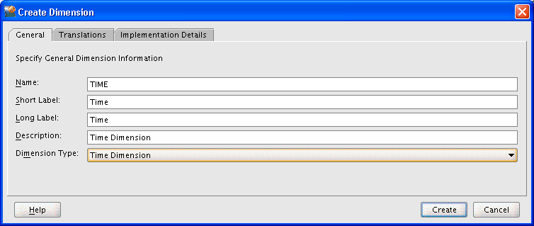
Figure 3-2 shows the creation of the Time dimension.
Figure 3-2 Creation of the Time Dimension
For business analysis, data is typically summarized by level. For example, your database may contain daily snapshots of a transactional database. Days are thus the base level. You might summarize this data at the weekly, quarterly, and yearly levels.
Levels have parent-child or one-to-many relationships, which form a level-based hierarchy. For example, each week summarizes seven days, each quarter summarizes 13 weeks, and each year summarizes four quarters. This hierarchical structure enables analysts to detect trends at the higher levels, then drill down to the lower levels to identify factors that contributed to a trend.
For each level that you define, you must identify a data source for dimension members at that level. Members at all levels are stored in the same dimension. In the previous example, the Time dimension contains members for weeks, quarters, and years.
Expand the folder for the dimension.
Right-click Levels, then choose Create Level.
The Create Level dialog box is displayed.
Complete all tabs of the Create Level dialog box.
Click Help for specific information about these choices.
Click Create.
The new level appears as an item in the Levels folder.
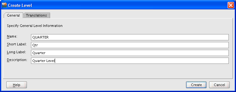
Figure 3-3 shows the creation of the Quarter level for the Time dimension.
Dimensions can have one or more hierarchies. Most hierarchies are level-based. Analytic Workspace Manager supports these common types of level-based hierarchies:
Normal hierarchies consist of one or more levels of aggregation. Members roll up into the next higher level in a many-to-one relationship, and these members roll up into the next higher level, and so forth to the top level.
Ragged hierarchies contain at least one member with a different base, creating a "ragged" base level for the hierarchy.
Skip-level hierarchies contain at least one member whose parents are multiple levels above it, creating a hole in the hierarchy. An example of a skip-level hierarchy is City-State-Country, where at least one city has a country as its parent (for example, Washington D.C. in the United States).
In relational source tables, a skip-level hierarchy may contain nulls in the level columns.
You may also have dimensions with parent-child relations that do not support levels. For example, an employee dimension might have a parent-child relation that identifies each employee's supervisor. However, levels that group together first-, second-, and third-level supervisors and so forth may not be meaningful for analysis. Similarly, you might have a line-item dimension with members that cannot be grouped into meaningful levels. In this situation, you can create a value-based hierarchy defined by the parent-child relations, which does not have named levels. You can create value-based hierarchies only for dimensions that use natural keys, because surrogate keys are formed with the names of the levels.
Expand the folder for the dimension.
Right-click Hierarchies, then choose Create Hierarchy.
The Create Hierarchy dialog box is displayed.
Complete all tabs of the Create Hierarchy dialog box.
If you define multiple hierarchies, be sure to define one of them as the default hierarchy.
Click Help for specific information about these choices.
Click Create.
The new hierarchy appears as an item in the Hierarchies folder.
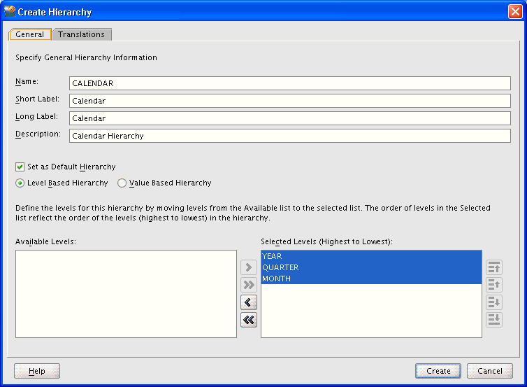
Figure 3-4 shows creation of the Calendar hierarchy for the Time dimension. Time has only one hierarchy, so Calendar is the default hierarchy.
Figure 3-4 Creation of the Calendar Hierarchy
Attributes provide information about the individual members of a dimension. They are used for labeling crosstabular and graphical data displays, selecting data, organizing dimension members, and so forth.
Analytic Workspace Manager creates some attributes automatically when creating a dimension. These attributes have a unique type, such as "Member Long Description," which OLAP client applications expect to find.
All dimensions are created with long and short description attributes. If your source tables include long and short descriptions, then you can map the attributes to the appropriate columns. However, if your source tables include only one set of labels, then you should always map the long description attributes. You can decide whether to map the short description attributes to the same column. If you do, the data is loaded twice.
Discoverer Plus OLAP, Spreadsheet Add-In, and OracleBI Beans use long description attributes in selection lists and for labeling crosstabs and graphs. The Add-In initially makes limited use of short description attributes, but users can switch to long descriptions. If the appropriate descriptions are not available, then these tools use dimension members. For example, if the Product dimension has short descriptions but no long descriptions, then the tools display Product dimension members.
Time dimensions are created with time-span and end-date attributes. This information must be provided for all Time dimension members.
Be sure to examine all of these attribute definitions, because you may wish to change the default settings. In particular, expand the hierarchy tree on the Basic tab to verify that the correct levels are selected. These choices affect the number of columns that you can map to the dimension.
You can create additional "User" attributes that provide supplementary information about the dimension members.
Expand the folder for the dimension.
Right-click Attributes, then choose Create Attribute.
The Create Attribute dialog box is displayed.
Complete all tabs of the Create Attribute dialog box.
Click Help for specific information about these choices.
Click Create.
The new attribute appears as an item in the Attributes folder.
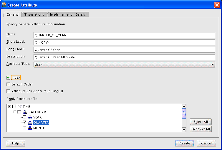
Figure 3-5 shows the creation of an attribute that pertains only to dimension members at the Quarter level of the Time dimension.
Figure 3-5 Creation of the Time Quarter of Year Attribute
Mapping identifies the relational data source for each dimensional object. After mapping a dimension to a column of a relational table or view, you can load the data. You can create, map, and load each dimension individually, or perform each step for all dimensions before proceeding to the next step.
The mapping window has a tabular view and a graphical view.
Tabular view. Drag-and-drop the names of individual columns from the schema navigation tree to the rows for the logical objects.
Graphical view. Drag-and-drop icons, which represent tables and views, from the schema navigation tree onto the mapping canvas. Then you draw lines from the columns to the logical objects.
Click Help on the Mapping page for more information. When you are done mapping the dimension, click Apply.
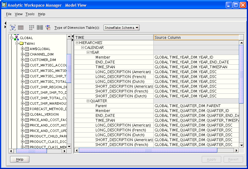
Figure 3-6 shows the TIME dimension mapped in the tabular view. The toolbar appears across the top and the schema navigation tree is on the left.
Figure 3-6 Time Dimension Mapped in a Tabular View
You can view the contents of a particular source column without leaving the mapping window. The information is readily available, eliminating the guesswork when the names are not adequately descriptive.
To see the values in a particular source table or view:
Right-click the source object in either the schema tree or the graphical view of the mapping canvas.
Choose View Data from the shortcut menu.
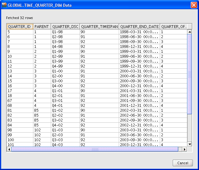
Figure 3-7 shows the data stored in the TIME_QUARTER_DIM table.
Figure 3-7 Data in a Source Dimension Table
Analytic Workspace Manager provides several ways to load data into dimensional objects. The quickest way when developing a data model is using the default choices of the Maintenance Wizard. Other methods may be more appropriate in a production environment than the one used here.
To load data into the dimensions:
In the navigation tree, right-click the Dimensions folder or the folder for a particular dimension, then choose Maintain Dimension.
The Maintenance Wizard opens on the Select Objects page.
Select one or more dimensions from Available Target Objects and use the shuttle buttons to move them to Selected Target Objects.
Click Finish to load the dimension values immediately.
The additional pages of the wizard enable you to create a SQL script or submit the load to the Oracle job queue. To use these options, click Next instead.
Review the build log, which appears when the build is complete. If the log shows that errors occurred, then fix them and run the Maintenance Wizard again.
Errors are typically caused by problems in the mapping. Check for incomplete mappings or changes to the source objects.
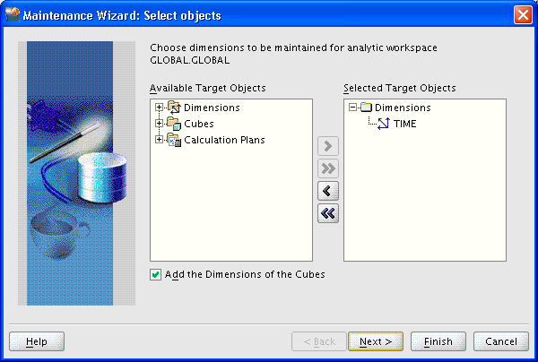
Figure 3-8 shows the first page of the Maintenance Wizard. Only the Time dimension has been selected for maintenance. All the Time dimension members and attributes are fetched from the mapped relational sources.
Figure 3-8 Loading Dimension Values into the Time Dimension
After loading a dimension, you can see its members by using the dimension viewer.
In the navigation tree, right-click the name of a dimension.
Choose View Data.
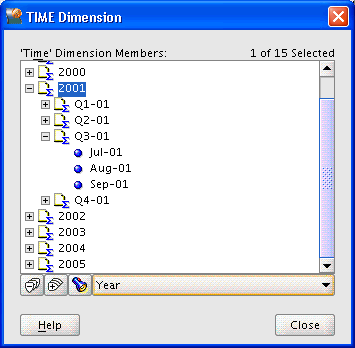
Figure 3-9 shows the Time dimension in the dimension viewer.
Cubes are informational objects that identify measures with the exact same dimensions and thus are candidates for being processed together at all stages: data loading, aggregation, storage, and querying.
Cubes define the shape of your business measures. They are defined by a set of ordered dimensions. The dimensions form the edges of a cube, and the measures are the cells in the body of the cube.
Expand the folder for the analytic workspace.
Right-click Cubes, then choose Create Cube.
The Create Cube dialog box is displayed.
Complete all tabs except Implementation Details of the Create Cube dialog box.
Important: After mapping the cube, run the Sparsity Advisor to see the recommended settings for the Implementation Details tab. For more information about the Summary To tab, refer to Chapter 8.
Click Create.
The new cube appears as a subfolder under Cubes.
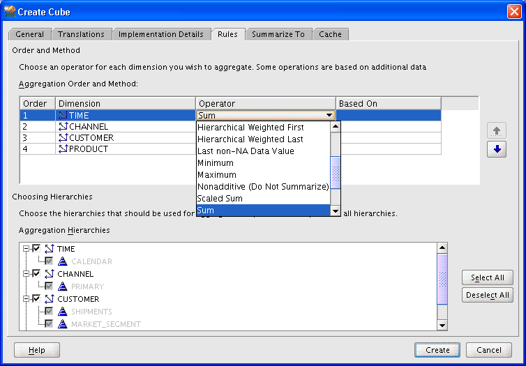
Figure 3-10 shows the Rules tab for the Units cube, with the list of aggregation operators displayed.
See Also:
For descriptions of the aggregation operators:Click Help on the Rules tab in Analytic Workspace Manager
Figure 3-10 Selecting an Aggregation Operator
Measures store the facts collected about your business. Each measure belongs to a particular cube, and thus shares particular characteristics with other measures in the cube, such as the same dimensions. The default attributes of a measure are inherited from the cube.
Expand the folder for the cube that has the dimensions of the new measure.
Right-click Measures, then choose Create Measure.
The Create Measure dialog box is displayed.
Complete the General tab of the Create Measure dialog box. Complete the other tabs to override the cube settings.
Click Create.
The new measure appears as an item in the Measures folder.
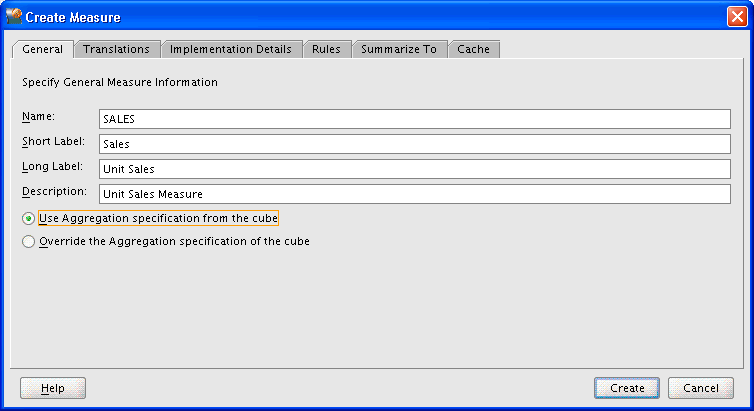
Figure 3-11 shows the General tab of the Create Measure dialog box.
You use the same interface to map cubes as you did to map dimensions, as described in "Mapping Dimensions".
To map a cube in the graphical view:
Define the cube and its measures.
In the navigation tree, expand the Cubes folder and click Mappings.
The Mapping Window is displayed in the right pane. You see a schema navigation tree and a table with rows for the measures, dimensions, and levels.
Enlarge the mapping window by dragging the divider to the left.
In the schema navigation tree, locate the tables with the measures. Drag-and-drop them onto the mapping canvas.
Draw lines from the source columns to the target objects.
To draw a line, click the output connector of the source column and drag it to the input connector of the target object. You must map both the measures and the related dimension keys.
To uncross the lines, click the Auto Arrange Mappings tool.
When you have mapped all objects for the dimension, drag the divider to the right to restore access to the navigation tree.
Figure 3-12 shows the mapping canvas with the Price and Cost cube mapped to columns in the PRICE_AND_COST_HIST_FACT table. The mapping toolbar is at the top, and the schema navigation tree is on the left.
Figure 3-12 Units Cube Mapped in Graphical View
The creation of a cube requires several decisions about data storage that affect the performance of the analytic workspace. These choices are on the Implementation Details tab for the cube. The Sparsity Advisor in Analytic Workspace Manager evaluates the data in the relational tables and recommends the appropriate settings. You can accept the recommendations or modify them before implementing them in the cube.
Partitioning is a method of physically storing the measures in a cube. It improves the performance of large measures in the following ways:
Improves scalability by keeping data structures small. Each partition functions like a smaller measure.
Keeps the working set of data smaller both for queries and maintenance, since the relevant data is stored together.
Enables parallel aggregation during data maintenance. Each partition can be aggregated by a separate process.
Simplifies removal of old data from storage. Old partitions can be dropped, and new partitions can be added.
The number of partitions affects the database resources that can be allocated to loading and aggregating the data in a cube. Partitions can be aggregated simultaneously when sufficient resources have been allocated.
The Sparsity Advisor analyzes the source tables and develops a partitioning strategy. You can accept the recommendations of the Sparsity Advisor, or you can make your own decisions about partitioning. Analytic Workspace Manager does not partition cubes by default.
If your partitioning strategy is driven primarily by life-cycle management considerations, then you should partition the cube on the Time dimension. Old time periods can then be dropped as a unit, and new time periods added as a new partition. In Figure 3-14, for instance, the Quarter level of the Time dimension is used as the partitioning key.
If life-cycle management is not a primary consideration, then partition on whatever dimension the Sparsity Advisor recommends. If the source fact table is partitioned, then the cube is partitioned on the same dimension. Otherwise, the Sparsity Advisor develops a strategy designed to achieve optimal build and query performance.
Create a cube and map it to a relational data source.
In the navigation tree, right-click the cube and choose Sparsity Advisor.
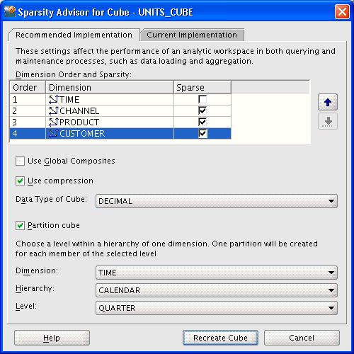
Wait while the Sparsity Advisor analyzes the cube. When it is done, the Sparsity Advisor for Cube dialog box displays the recommendations.
For compressed cubes, be sure to select a data type for the cube.
Look over the recommendations and make any changes.
Click Recreate Cube to implement the recommendations.
Figure 3-13 shows the Sparsity Advisor dialog box with settings that are typical for a real-world cube.
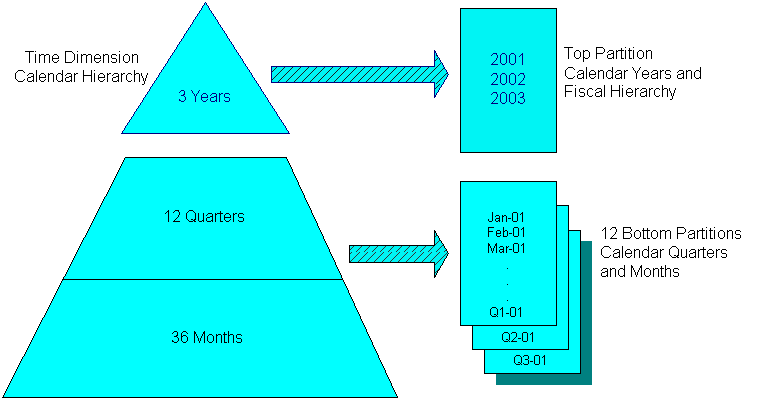
The Partitioning Advisor might recommend partitioning at the Quarter level of the Calendar hierarchy of the Time dimension. Each Quarter and its descendants are stored in a separate partition. If there are three years of data in the analytic workspace, then partitioning on Quarter produces 12 bottom partitions, in addition to the default top partition. The top partition contains all remaining levels, that is, those above Quarter (such as Year) and those in other hierarchies (such as Fiscal Year or Year-to-Date).
Figure 3-14 illustrates a Time dimension partitioned by Quarter.
You load data into cubes using the same methods as dimensions. However, loading and aggregating the data for your business measures typically takes more time to complete. Unless you are developing a dimensional model using a small sample of data, you may prefer to run the build in one or more background processes.
In the navigation tree, right-click the Cubes folder or the name of a particular cube.
Choose Maintain Cube.
The Maintenance Wizard opens on the Select Objects page.
Select one or more cubes from Available Target Objects and use the shuttle buttons to move them to Selected Target Objects. If the dimensions are already loaded, you can omit them from Selected Target Objects.
On the Dimension Data Processing Options page, you can choose to do a complete or a partial refresh of the cube.
On the Task Processing Options page, you can submit the build to the Oracle job queue or create a SQL script that you can run outside of Analytic Workspace Manager.
You can also select the number of processes to dedicate to this build. The number of parallel processes is limited by the smallest of these numbers: The number of partitions in the cube, the number of processes dedicated to the build, and the setting of the JOB_QUEUE_PROCESSES initialization parameter.
Click Help for information about these choices.
Click Finish.
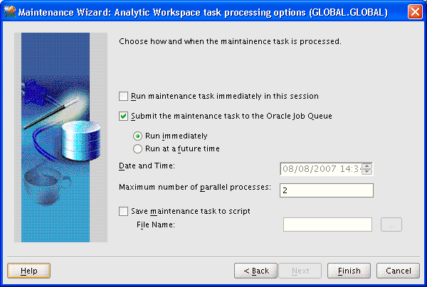
Figure 3-15 shows the build submitted immediately to the Oracle job queue.
Figure 3-15 Selecting the Task Processing Options
After loading a cube, you can display the data for your business measures in Analytic Workspace Manager.
To display the data in a cube:
In the navigation tree, right-click the cube.
Choose View Data from the shortcut menu.
The Measure Data Viewer displays the selected measure in a crosstab at the top of the page and a graph at the bottom of the page. On the crosstab, you can expand and collapse the dimension hierarchies that label the rows and columns. You can also change the location of a dimension by pivoting or swapping it. If you wish, you can use multiple dimensions to label the columns and rows, by nesting one dimension under another.
To pivot, drag a dimension from one location and drop it at another location, usually above or below another dimension.
To swap dimensions, drag and drop one dimension directly over another dimension, so they exchange locations.
To make extensive changes to the selection of data, choose Query Builder from the File menu.
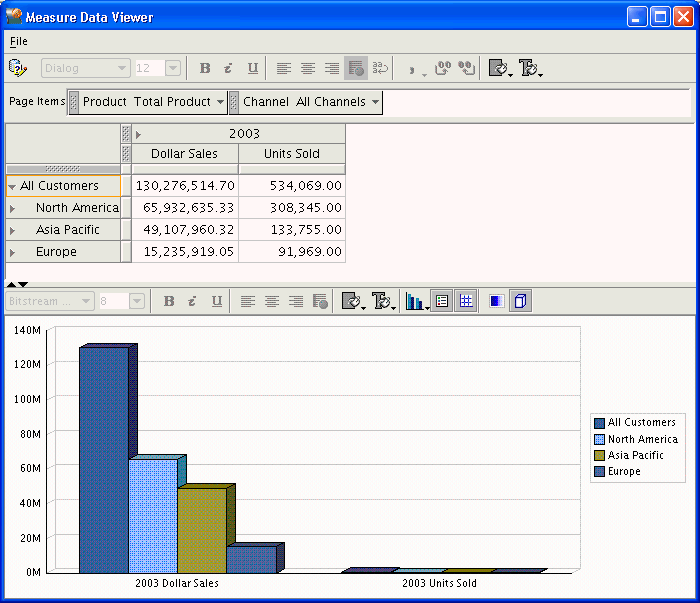
Figure 3-16 shows the Units cube in the Measure Viewer.
You can define a measure folder for use by OLAP tools, so that the measures can be located and identified quickly by users. They may have access to several analytic workspaces or relational schemas with measures named Sales or Costs, and they have no means of differentiating them outside of a measure folder. The Cube Viewer in Analytic Workspace Manager also uses measure folders.
Expand the folder for the analytic workspace.
Right-click Measure Folders, then choose Create Measure Folder.
Complete the General tab of the Create Measure Folder dialog box.
Click Help for specific information about these choices.
The new measure folder appears in the navigation tree under Measure Folders. You can also create subfolders.
Figure 3-17 shows creation of a measure folder.
A single analytic workspace can support multiple languages. This support enables users of OLAP applications and tools to view the metadata in their native languages. For example, you can provide translations for the display names of measures, cubes, and dimensions. You can also map attributes to multiple columns, one for each language.
The number and choice of languages is restricted only by the database character set and your ability to provide translated text. Languages can be added or removed at any time.
To add support for multiple languages:
In the navigation tree, expand the folder for the analytic workspace.
Click Languages and select the languages for the analytic workspace on the Basic tab.
For each dimension, level, hierarchy, attribute, cube, measure, calculated measure, and measure folder, select the Translations tab of the property sheet. Enter the object labels and descriptions in each language.
For each dimension, open the Mappings window. Map the attributes to columns for each language.
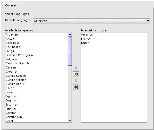
Figure 3-18 shows the selection of languages.
Analytic Workspace Manager enables you to save all or part of the multidimensional model as a text file. This text file contains the XML definitions of the dimensional objects, such as dimensions, levels, hierarchies, attributes, and measures. Only the metadata is saved, not the data or any customizations. Templates are small files, so you can easily distribute them by e-mail or on a Web site, just as the templates for Global and Sales History are distributed on the Oracle Web site. To re-create the logical objects, you simply identify the templates in Analytic Workspace Manager.
You can save the following types of objects as XML templates:
Analytic workspace: Saves all logical objects. You can save measure folders and calculation plans only by saving the complete analytic workspace.
Cube: Saves the cube and its measures, calculated measures, and mappings.
Calculated measure: Saves just the calculated measure.
Dimension: Saves the dimension and its levels, hierarchies, attributes, and mappings.
In the navigation tree, right-click the object and choose Save object to Template.
To create logical objects from a template:
In the navigation tree, right-click the object type and choose Create object From Template.
|
Copyright © 2003, 2012, Oracle and/or its affiliates. All rights reserved. Legal Notices |
|